Forecast Revisions with TimeDB
This notebook demonstrates overlapping forecast revisions:
Creating multiple forecasts for the same series with different
known_timeReading all revisions with
read(versions=True)Visualizing how forecasts evolve over time
[1]:
from timedb import TimeDataClient
import pandas as pd
import numpy as np
from datetime import datetime, timedelta, timezone
import matplotlib.pyplot as plt
from dotenv import load_dotenv
load_dotenv()

td = TimeDataClient()
td.delete()
td.create()
Creating database schema...
✓ Schema created successfully
[2]:
forecast_series_id = td.create_series(
    name='forecast',
    unit='MW',
    labels={'type': 'power_forecast', 'model': 'sinus_with_error'},
    description='Forecasted power values with overlapping revisions',
    overlapping=True
)

observation_series_id = td.create_series(
    name='flat',
    unit='MW',
    labels={'type': 'power_observation'},
    description='Observation power values (ground truth)'
)

for s in td.series().list_series():
    print(f"  {s['name']}: unit={s['unit']}  overlapping={s['overlapping']}  labels={s['labels']}")
  flat: unit=MW  overlapping=False  labels={'type': 'power_observation'}
  forecast: unit=MW  overlapping=True  labels={'type': 'power_forecast', 'model': 'sinus_with_error'}
Part 2: Create 4 Forecasts with Shifting Valid Times
Each forecast has a 3-day (72h) horizon starting at its known_time, with forecasts issued 1 day apart. Forecast error grows with lead time — early hours are accurate, later hours diverge.
[3]:
base_valid_time = datetime(2025, 1, 1, 0, 0, tzinfo=timezone.utc)
forecast_horizon_hours = 72
num_forecasts = 4

# Generate "observation" power values over the full period (diurnal pattern + noise)
np.random.seed(0)
total_hours = (num_forecasts - 1) * 24 + forecast_horizon_hours
all_hours = np.arange(total_hours)
observations = 80 + 40 * np.sin(2 * np.pi * all_hours / 24 - np.pi / 2) + np.random.normal(0, 3, total_hours)
observations = np.clip(observations, 0, None)  # power can't be negative

# Insert 4 forecasts — each starts at its known_time, error grows with lead time
for i in range(num_forecasts):
    known_time = base_valid_time + timedelta(days=i)
    start_idx = i * 24  # offset into observations array
    valid_times = [known_time + timedelta(hours=j) for j in range(forecast_horizon_hours)]
    lead_hours = np.arange(forecast_horizon_hours)
    np.random.seed(42 + i)
    forecast_error = np.random.normal(0, 1 + 0.3 * lead_hours)
    forecast_values = np.round(observations[start_idx:start_idx + forecast_horizon_hours] + forecast_error, 2)

    df_forecast = pd.DataFrame({"valid_time": valid_times, "value": forecast_values})
    td.series("forecast").where(type='power_forecast', model='sinus_with_error').insert(
        df=df_forecast, known_time=known_time
    )

# Insert observation values
observation_valid_times = [base_valid_time + timedelta(hours=i) for i in range(total_hours)]
df_observation = pd.DataFrame({"valid_time": observation_valid_times, "value": np.round(observations, 2)})
td.series("flat").where(type='power_observation').insert(df=df_observation)

print(f"Inserted {num_forecasts} forecast batches + observations ({total_hours} hours)")
Inserted 4 forecast batches + observations (144 hours)
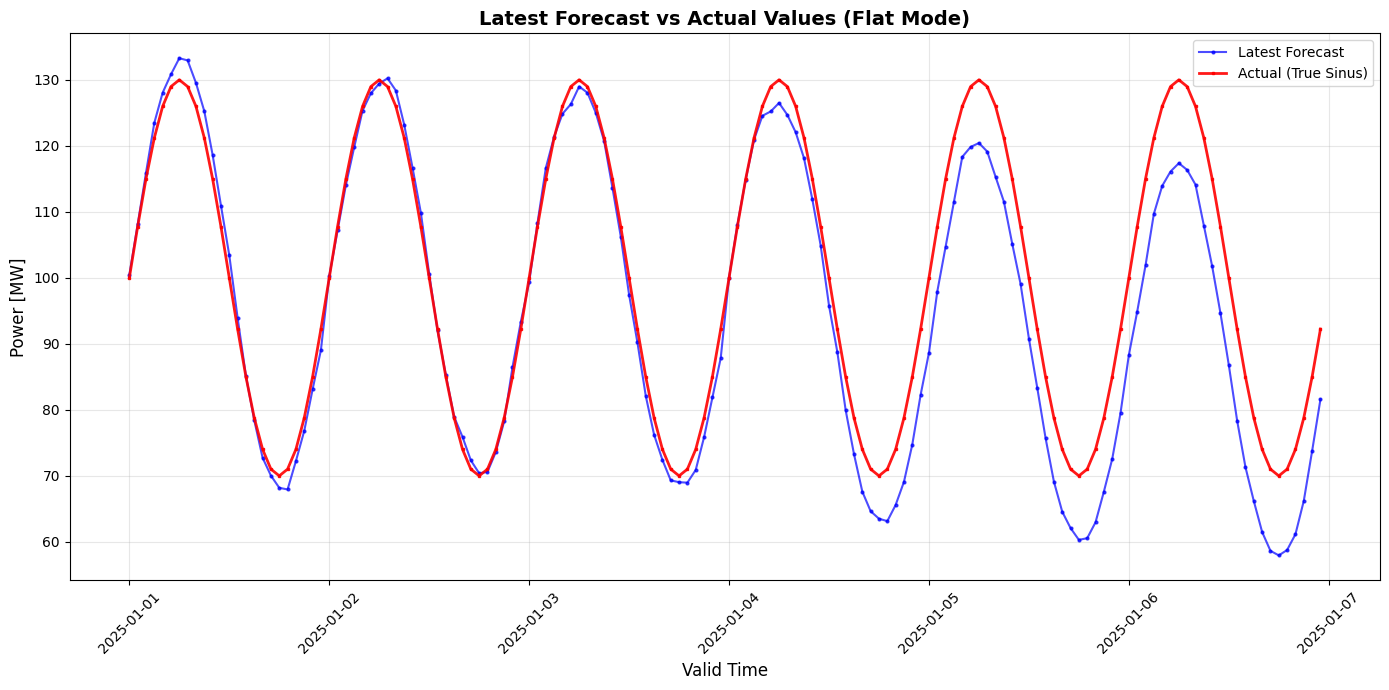
Part 3: Read Latest Forecast Revisions
Now we’ll read back the latest forecast revisions using td.read(). This returns the latest forecast for each valid_time (most recent based on known_time) in a single query. The observations are recorded in a separate series.
[4]:
start_valid = base_valid_time
end_valid = base_valid_time + timedelta(hours=total_hours)

# Read latest forecast and observations
df_forecast = td.series("forecast").where(
    type='power_forecast', model='sinus_with_error'
).read(start_valid=start_valid, end_valid=end_valid)

df_observation = td.series("flat").where(
    type='power_observation'
).read(start_valid=start_valid, end_valid=end_valid)

df_flat = pd.DataFrame({
    'forecast': df_forecast['value'],
    'observation': df_observation['value']
}, index=df_forecast.index)

df_flat.head(10)
[4]:
| forecast | observation | |
|---|---|---|
| valid_time | ||
| 2025-01-01 00:00:00+00:00 | 45.79 | 45.29 |
| 2025-01-01 01:00:00+00:00 | 42.38 | 42.56 |
| 2025-01-01 02:00:00+00:00 | 49.33 | 48.30 |
| 2025-01-01 03:00:00+00:00 | 61.33 | 58.44 |
| 2025-01-01 04:00:00+00:00 | 65.09 | 65.60 |
| 2025-01-01 05:00:00+00:00 | 66.13 | 66.72 |
| 2025-01-01 06:00:00+00:00 | 87.27 | 82.85 |
| 2025-01-01 07:00:00+00:00 | 92.28 | 89.90 |
| 2025-01-01 08:00:00+00:00 | 98.09 | 99.69 |
| 2025-01-01 09:00:00+00:00 | 111.52 | 109.52 |
[5]:
fig, ax = plt.subplots(figsize=(14, 5))

ax.plot(df_flat.index, df_flat['observation'].astype(float), linewidth=2, color='#2ca02c', label='Observation', zorder=5)
ax.plot(df_flat.index, df_flat['forecast'].astype(float), linewidth=1.5, color='steelblue', label='Latest Forecast', alpha=0.8)

ax.set_xlabel('Valid Time')
ax.set_ylabel('Power [MW]')
ax.set_title('Latest Forecast vs Observation')
ax.legend()
ax.grid(True, alpha=0.3)
fig.autofmt_xdate()
plt.tight_layout()
plt.show()
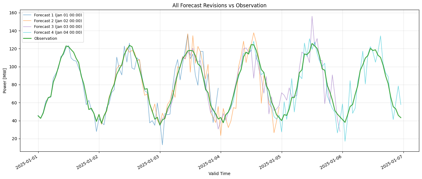
Part 4: Read All Forecast Revisions (Overlapping Mode)
Now let’s read all forecast revisions using .read(versions=True) on the series collection. This returns all forecasts with both known_time and valid_time, showing how forecasts evolve over time. This is useful for analyzing forecast revisions and backtesting.
[6]:
# Read all forecast revisions with (known_time, valid_time) multi-index
df_forecast_overlapping = td.series("forecast").where(
    type='power_forecast', model='sinus_with_error'
).read(start_valid=start_valid, end_valid=end_valid, versions=True)

# Read observations (flat)
df_observation_overlapping = td.series("flat").where(
    type='power_observation'
).read(start_valid=start_valid, end_valid=end_valid)

print(f"Forecast: {df_forecast_overlapping.shape}  index={df_forecast_overlapping.index.names}")
print(f"Observation:   {df_observation_overlapping.shape}  index={df_observation_overlapping.index.name}")
print()
df_forecast_overlapping.head(6)
Forecast: (288, 1)  index=['known_time', 'valid_time']
Observation:   (144, 1)  index=valid_time
[6]:
| value | ||
|---|---|---|
| known_time | valid_time | |
| 2025-01-01 00:00:00+00:00 | 2025-01-01 00:00:00+00:00 | 45.79 |
| 2025-01-01 01:00:00+00:00 | 42.38 | |
| 2025-01-01 02:00:00+00:00 | 49.33 | |
| 2025-01-01 03:00:00+00:00 | 61.33 | |
| 2025-01-01 04:00:00+00:00 | 65.09 | |
| 2025-01-01 05:00:00+00:00 | 66.13 |
[7]:
fig, ax = plt.subplots(figsize=(14, 6))

# Plot each forecast revision in a distinct color
unique_known_times = df_forecast_overlapping.index.get_level_values("known_time").unique()
colors = ['#1f77b4', '#ff7f0e', '#9467bd', '#17becf']

for idx, known_time in enumerate(unique_known_times):
    forecast_data = df_forecast_overlapping.xs(known_time, level="known_time")
    values = forecast_data['value'].astype(float)
    label = f"Forecast {idx+1} ({known_time.strftime('%b %d %H:%M')})"
    ax.plot(forecast_data.index, values, linewidth=1.2,
            color=colors[idx % len(colors)], alpha=0.6, label=label)

# Plot observations on top
observation_vals = df_observation_overlapping['value'].astype(float)
ax.plot(df_observation_overlapping.index, observation_vals, linewidth=2,
        color='#2ca02c', label='Observation', alpha=0.9, zorder=10)

ax.set_xlabel('Valid Time')
ax.set_ylabel('Power [MW]')
ax.set_title('All Forecast Revisions vs Observation')
ax.legend(fontsize=9)
ax.grid(True, alpha=0.3)
fig.autofmt_xdate()
plt.tight_layout()
plt.show()
Summary
known_time= when the forecast was made;valid_time= what it predictsoverlapping=Trueenables versioned storage withknown_timetrackingread()returns the latest forecast (one value pervalid_time)read(versions=True)returns all revisions with a(known_time, valid_time)multi-index